Andrew Abok Follow

Implied Volatility Model.

Have you ever wondered why options prices can vary so much, even when the underlying asset’s price hasn’t changed? The answer lies in a powerful concept called implied volatility. Today, we’ll explore what implied volatility is, why it matters, and how it’s calculated using models like Black-Scholes

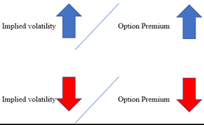
Implied volatility is a metric that reflects the market’s expectation of how much a security or asset’s price will move in the future. It’s derived from the price of options.

The volatility smile effect is an empirical fact that the BSM model fails to explain.

Unlike the flat volatility surface assumed by the Black-Scholes model, real-world markets often exhibit higher implied volatilities for options that are far out-of-the-money (OTM) or in-the-money (ITM). This creates a ‘smile’ shape when plotted. For example, during times of market uncertainty, out-of-the-money put options tend to have higher implied volatilities because investors are willing to pay a premium for protection against downside risk.This is among the limitations of the BSM model.

Let’s define the market dynamics: The security price.

d S_{t} = μ S_{t} d_{t} + σ W_{t}

The price of the standard European call option:

C = C (σ, K, T) = S_{0} ϕ (d_{1}) - K e^{- r T} ϕ (d_{2})

we will define The actual market prices as $\hat{C} (T, K)$

having both the BSM price and the actual market price We can now compare $C (σ, T, K)$ with $\hat{C} (T, K)$ and define the implied volatility $\hat{σ}$ as the solution to:

f (σ) = C (σ, T, K) - \hat{C} (T, K)

Newton-Rhapson

Newton’s method is an iterative update rule for finding the roots of an equation $f (x) = 0$ .

X_{i + 1} = X_{i} - \frac{f (X_{i})}{f^{'} (X_{i})}

For an arbitrary equation where computing the derivative $f^{'} (x)$ is difficult one can use the finite difference approximation

f^{'} (x) = \frac{f (x + ϵ) - f (x)}{ϵ}

We can use Newton-Rhapson to find the solution for the Implied volatility problem.

With Newton’s method being an iterative method; we are trying to solve

f (σ, S, K, r, T - t) - C = 0,

from an initial guess $σ_{0}$ , we form the Newton iterates

σ_{n} = σ_{n - 1} - \frac{f (σ_{n - 1})}{f^{'} (σ_{n - 1})}

Using Newton’s method means we have to differentiate the Black-Scholes formula with respect to sigma. This derivative is the vega for a European call option is

f^{'} (σ) = S ϕ (d_{1}) \sqrt{T - t} e x p (- r (T - t))

In practice $\hat{σ} = σ (T, K)$ is not constant.

Changes with T for fixed K and
Changes with K for fixed T as a convex function (hence the name smile effect). This change appears to be more delicate.

BSM model assumes constant volatility which is not true.

Volatility surface

The Black-Scholes model implies that $I (K, T) = σ$ a flat volatility surface for all K and T

Some key observation of the volatility surface is that:

Options of lowerstrikes tend to have higher implied volatilities
For a given maturity T, this feature is called volatility skew or volatility smile
For a given strike, K, the implied volatility can be either increasing or decreasing with T

In general, $I (K, T) \to σ, T \to \infty$

As $T \to 0$ , we observe an inverted volatility surface where short-term options have higher volatilities when compared with long-term options

Implementation in Python

from scipy.stats import norm    
import matplotlib.pyplot as plt
import numpy as np
import matplotlib.pyplot as plt
from mpl_toolkits.mplot3d import Axes3D
from scipy.interpolate import griddata
import pandas as pd  


#Define the BSM Call Function.
def europeanCallOptionPrice(S, K, r, sigma, T):
    d1 = (np.log(S / K) + (r + 0.5 * sigma**2) * (T)) / (sigma * np.sqrt(T))
    d2 = d1 - (sigma * np.sqrt(T))
    
    callPrice = S * norm.cdf(d1) - (K * np.exp(-r * T) * norm.cdf(d2))
    return callPrice

#Define Vega the deriviative of the BSM with respect to sigma.
def vega(S, K, r, sigma, T):
    d1 = (np.log(S / K) + (r + 0.5 * sigma**2) * T) / (sigma * np.sqrt(T))
    vega = S * np.sqrt(T) * norm.pdf(d1) * np.exp(-r *T)
    return vega


#Define the implied volatility function.
def impliedVolatility(currentCallPrice, S, K, r,T, maxIter=10000):
    sigma = 0.15
    tolerance = 0

    for i in range(maxIter):
        optionPrice = europeanCallOptionPrice(S, K, r, sigma, T)
        derivative = vega(S, K, r, sigma, T)
        #Objective function. - the diffrence between the call price with the initali call price.
        diff = optionPrice - currentCallPrice

        if diff == tolerance:
            sigma = sigma

        sigma -= diff / derivative        

    return sigma
    
    
T = [0.25, 0.5, 1.0, 1.5]
K = [60, 70, 80, 90, 100, 110, 120, 130, 140]

#Initiate the matrix.
VolatilitySurfaceMatrix = [[0 for _ in range(len(T))] for _ in range(len(K))]

S = 100
r = 0.03
sigma = 0.05

for i in range(len(K)):
    for j in range(len(T)):
        k = K[i]
        t = T[j]
        C = europeanCallOptionPrice(S, k, r, sigma, t)
        VolatilitySurfaceMatrix[i][j] = impliedVolatility(C, S, k, r,t)
VolatilitySurfaceMatrix

#Create a meshgrid for strike prices and maturities
T_mesh, K_mesh = np.meshgrid(T, K)

#Convert the surface matrix to a numpy array
VolatilitySurfaceMatrix = np.array(VolatilitySurfaceMatrix)

#Create a 3D plot
fig = plt.figure()
ax = fig.add_subplot(111, projection='3d')

#Plot the surface
ax.plot_surface(K_mesh, T_mesh, VolatilitySurfaceMatrix, cmap='viridis')

#Set labels and title
ax.set_xlabel('Strike Price')
ax.set_ylabel('Maturity')
ax.set_zlabel('Implied Volatility')
ax.set_title('Implied Volatility Surface')

# Show the plot
plt.show()


VolatilitySurfaceMatrix = np.array(VolatilitySurfaceMatrix)

# Set up the desired grid for interpolation
TInterp = np.linspace(min(T), max(T), 100)
KInterp = np.linspace(min(K), max(K), 100)
TInterpMesh, KInterpMesh = np.meshgrid(TInterp, KInterp)

# Perform linear interpolation on the surface matrix
VolatilitySurfaceMatrix_interp = griddata((T_mesh.flatten(), K_mesh.flatten()), VolatilitySurfaceMatrix.flatten(),
                                          (TInterpMesh,KInterpMesh), method='linear')

# Create a 3D plot
fig = plt.figure()
ax = fig.add_subplot(111, projection='3d')

# Plot the interpolated surface
ax.plot_surface(KInterpMesh,TInterpMesh, VolatilitySurfaceMatrix_interp, cmap='viridis')

# Set labels and title
ax.set_xlabel('Strike Price')
ax.set_ylabel('Maturity')
ax.set_zlabel('Implied Volatility')
ax.set_title('Implied Volatility Surface (Interpolated)')

# Show the plot
plt.show()

Refrences

https://www.kent.ac.uk/learning/documents/slas-documents/implied-volatility.pdf

03 Mar 2025

Software Development

« ETL AND ELT Optimizing Pattern Matching in F# for Better Performance »